Reproducibility

Every figure is computed, not drawn

A scientific reference should be checkable. The quantitative figures tied to P(t) on this site are generated by code you can run yourself, and the illustrative aggregate estimate comes from a Monte-Carlo procedure with a fixed random seed. This page shows the two core figures as selectable vector graphics and links the notebook that regenerates them.

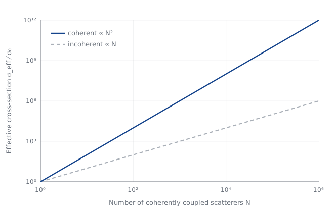
The parameter magnitudes used below are illustrative order-of-magnitude placeholders, flagged as such — they exercise the method, they are not measured device specifications. What is reproducible here is the machinery: the scaling laws, the numerics, and the convergence.

Coherent enhancement: the N² law

When many constituents respond in phase, scattering amplitudes add and the effective cross-section scales as the square of their number, N², rather than linearly. This is the mechanism that lifts a tiny per-particle cross-section to macroscopic relevance, developed in the cross-section and deep-dive chapters. The figure contrasts the coherent N² scaling with incoherent linear scaling on log–log axes.

Log–log plot of effective cross-section against the number of coherently coupled scatterers N, showing coherent scaling proportional to N squared as a solid line and incoherent scaling proportional to N as a dashed line. — Effective cross-section versus the number of coherently coupled scatterers. The coherent branch (solid) has slope 2; the incoherent branch (dashed) has slope 1.

Monte-Carlo convergence of the aggregate

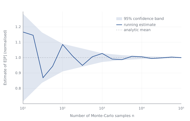
P(t) is a product of factors, each uncertain across an order of magnitude. Modelling each factor as log-normal, we estimate the mean of the product by Monte-Carlo. Because the mean of a product of log-normals is available in closed form, we can check that the estimator is unbiased: the running estimate converges onto the analytic mean and its 95% confidence band shrinks as 1/√n. This complements the Monte-Carlo validation and sigma analysis chapters.

Semi-logarithmic plot of the Monte-Carlo estimate of the mean output, normalised to the analytic mean, against the number of samples, showing the running estimate converging to one inside a shrinking 95 percent confidence band. — Running Monte-Carlo estimate of the aggregate (normalised to the analytic mean), with its 95% confidence band narrowing as the sample count grows.

Reproduce it yourself

The notebook below regenerates both figures and prints the Monte-Carlo estimate against the analytic mean. It has a fixed seed, so results are identical run to run, and depends only on numpy and matplotlib.

Download the notebook — pt-schubart-reproducibility.ipynb →

Run with pip install numpy matplotlib then open in Jupyter, or execute headless with jupyter nbconvert --execute.